Tutorial¶

This tutorial mirrors the package vignette. It uses the bundled example repertoire samples_db (several individuals of IGH AIRR-seq data) and the bundled germline references.

library(rabhit)
data(samples_db, HVGERM, HDGERM)

Haplotype inference by an anchor gene¶

J gene anchor (IGHJ6)¶

Roughly one third of individuals are heterozygous at IGHJ6, which makes it a natural anchor.

clip_db <- samples_db[samples_db$subject == "I5", ]

haplo_db_J6 <- createFullHaplotype(clip_db,
                                   toHap_col = c("v_call", "d_call"),
                                   hapBy_col = "j_call", hapBy = "IGHJ6",
                                   toHap_GERM = c(HVGERM, HDGERM))
head(haplo_db_J6, 3)

Plot the haplotype map:

plotHaplotype(haplo_db_J6)

Single-subject haplotype map

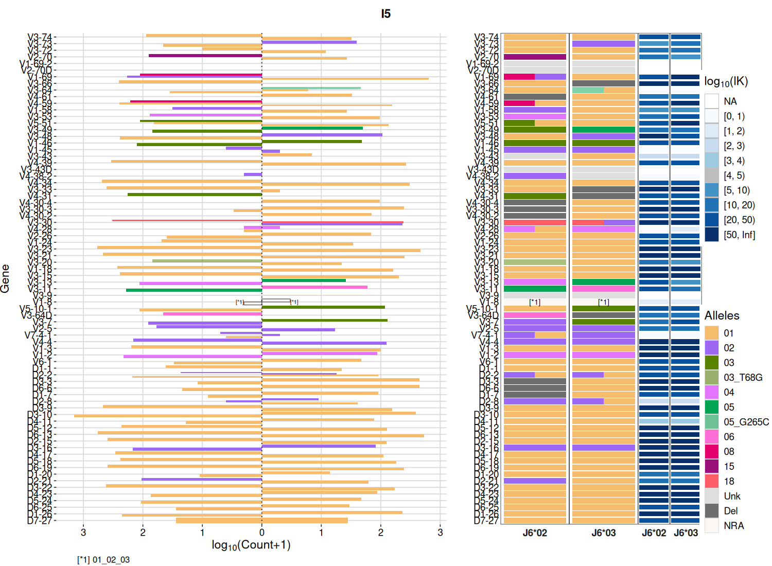
The left panel shows per-gene read counts, the middle panels the allele frequencies on each chromosome (one column per anchor allele), and the right panels the Bayes factor lK for each assignment.

D gene anchor (IGHD2-21)¶

Any sufficiently heterozygous gene can be used as the anchor:

haplo_db_D2_21 <- createFullHaplotype(clip_db,
                                      toHap_col = "v_call",
                                      hapBy_col = "d_call", hapBy = "IGHD2-21",
                                      toHap_GERM = HVGERM)

Tip

The anchor must be heterozygous with exactly two alleles, each above min_minor_fraction (default 0.3). Samples that do not meet this are reported and skipped.

Visualizing multiple samples¶

Infer haplotypes for several subjects, then draw a heatmap. hapHeatmap returns the plot together with an optimal width/height for rendering:

clip_dbs <- samples_db[samples_db$subject != "I5_FR2", ]
haplo_db <- createFullHaplotype(clip_dbs,
                                toHap_col = c("v_call", "d_call"),
                                hapBy_col = "j_call", hapBy = "IGHJ6",
                                toHap_GERM = c(HVGERM, HDGERM))

p.list <- hapHeatmap(haplo_db)
p.list$p          # the plot
p.list$width      # suggested width
p.list$height     # suggested height

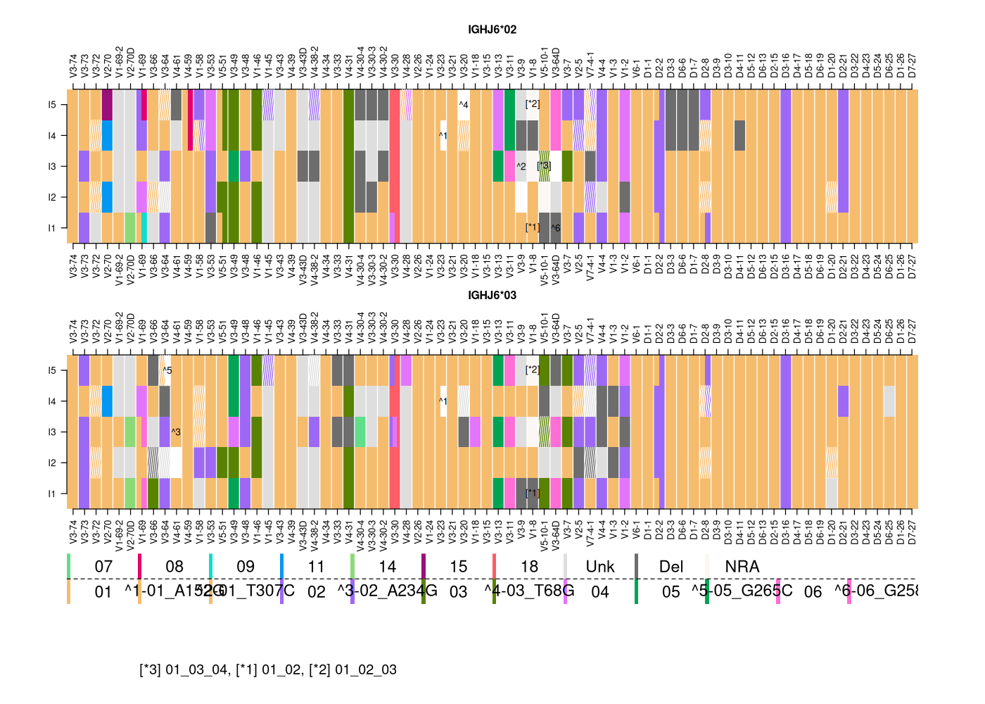
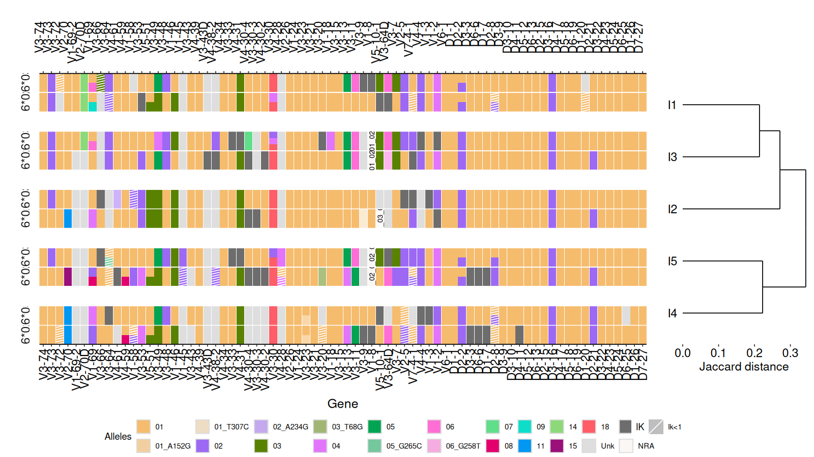
Haplotype heatmap across subjects

A dendrogram clusters samples by haplotype similarity (Jaccard distance). This needs the optional ggdendro package:

hapDendo(haplo_db)

Haplotype dendrogram

Deletion inference¶

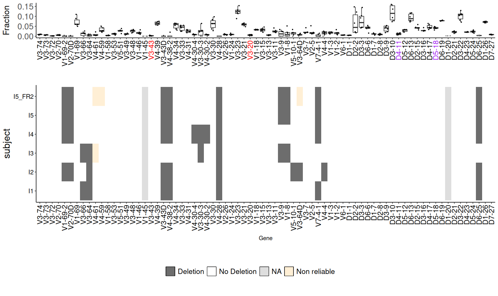
Double-chromosome deletions (binomial test)¶

del_binom_db <- deletionsByBinom(clip_dbs)
del_binom_db <- del_binom_db[grep("IGHJ", del_binom_db$gene, invert = TRUE), ]
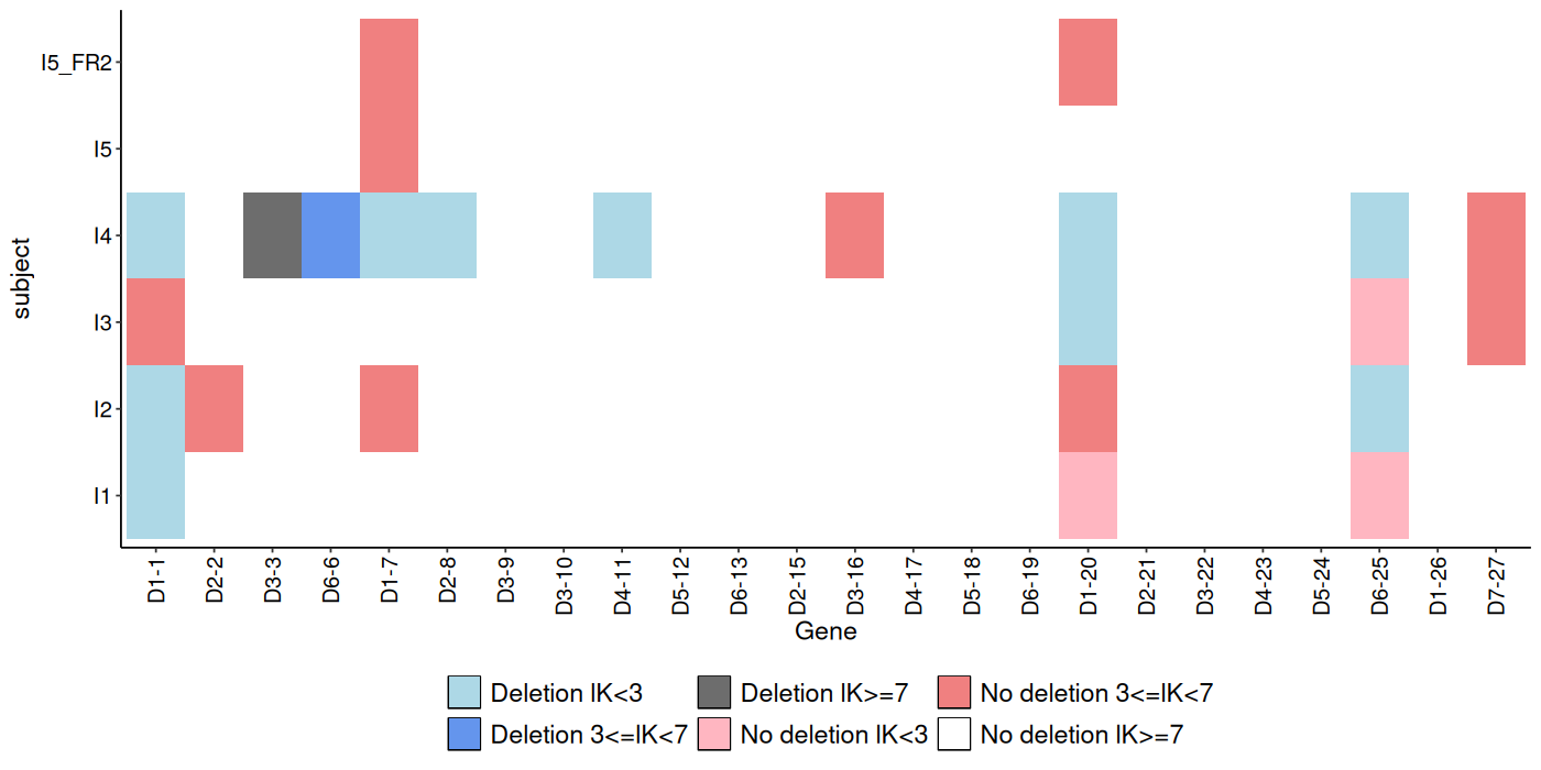
plotDeletionsByBinom(del_binom_db)

Double-chromosome deletions

Single-chromosome deletions (V pooled)¶

nonReliable_Vgenes <- nonReliableVGenes(samples_db)
del_db <- deletionsByVpooled(samples_db, nonReliable_Vgenes = nonReliable_Vgenes)
head(del_db)
plotDeletionsByVpooled(del_db)

Single-chromosome V deletions

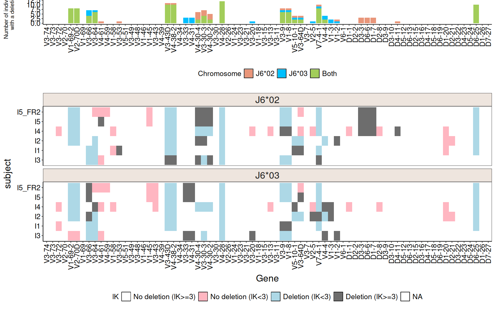
Deletion heatmap across subjects¶

del_binom_db <- deletionsByBinom(samples_db, nonReliable_Vgenes = nonReliable_Vgenes)
haplo_db <- createFullHaplotype(samples_db,
                                toHap_col = c("v_call", "d_call"),
                                hapBy_col = "j_call", hapBy = "IGHJ6",
                                toHap_GERM = c(HVGERM, HDGERM),
                                deleted_genes = del_binom_db,
                                nonReliable_Vgenes = nonReliable_Vgenes)
deletionHeatmap(haplo_db)

Deletion heatmap across subjects

Handling partial V coverage¶

For datasets with partial V coverage (e.g. primer-limited protocols), detect non-reliable V genes and feed them — together with detected deletions — back into the haplotype inference:

clip_db <- samples_db[samples_db$subject == "I5_FR2", ]
nonReliable_Vgenes <- nonReliableVGenes(clip_db)
del_binom_db <- deletionsByBinom(clip_db, chain = "IGH",
                                 nonReliable_Vgenes = nonReliable_Vgenes)

haplo_db <- createFullHaplotype(clip_db,
                                toHap_col = c("v_call", "d_call"),
                                hapBy_col = "j_call", hapBy = "IGHJ6",
                                toHap_GERM = c(HVGERM, HDGERM),
                                deleted_genes = del_binom_db,
                                nonReliable_Vgenes = nonReliable_Vgenes)

Interactive output¶

Set html_output = TRUE to obtain an interactive HTML5 plot (requires plotly and htmlwidgets):

p <- plotHaplotype(hap_table = haplo_db, html_output = TRUE)
htmlwidgets::saveWidget(p, "haplotype.html", selfcontained = TRUE)